② Parameters tab

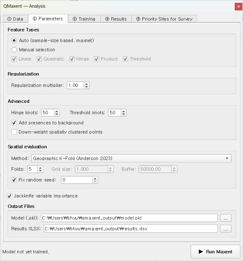
The Parameters tab controls the modeling and evaluation settings: which Maxent feature classes to allow, the regularization multiplier, the spatial cross-validation method, and where to write outputs. Defaults follow established Maxent practice; this chapter explains what each control does and when to override the default.

Feature Types

Maxent's "features" are the basis functions it uses to express the response of suitability to each environmental variable (Phillips, Anderson & Schapire 2006; Phillips et al. 2017). The five classes (LQPHT) are:

Feature	Symbol	What it captures
Linear	L	Monotonic linear response
Quadratic	Q	Optimum-shaped (∩) or U-shaped (∪) response
Product	P	Pairwise interactions between two variables
Hinge	H	Piecewise-linear "kink" — sharp changes at threshold values
Threshold	T	Step-function — a hard cut-off at some value

QMaxent offers two modes:

• Auto (default) — applies the Phillips & Dudík 2008 sample-size rule used by maxnet: L only for ≤10 presences, L+Q for ≤30, L+Q+H for ≤80, and L+Q+P+H+T above 80. This is the single most extensively benchmarked rule in the Maxent literature and is the safe default.
• Manual — pick any subset of LQPHT explicitly. Useful only when you are reproducing a published study that fixed a particular feature combination (e.g. the Pitta nympha example fixes feature classes to LQH to match Lee et al. 2025).

When in doubt, leave it on Auto

Repeatedly tuning feature classes without spatially-blocked CV is the primary source of optimistic AUCs flagged by Roberts et al. 2017. The auto rule sidesteps that failure mode entirely.

Regularization multiplier

Maxent fits a regularized maximum-entropy distribution — the regularization multiplier (RM) controls how strongly the fit is penalised for complexity. - RM = 1 (default) — the value Phillips & Dudík 2008 showed yields the best held-out AUC across the full Maxent benchmark. - RM > 1 (e.g. 2–4) — smoother responses, less over-fit, lower training AUC but often higher CV AUC. Use when occurrences are small in number, spatially clustered, or biased. - RM < 1 — only justified by a formal hyperparameter search such as ENMeval (Muscarella et al. 2014) or Wallace (Kass et al. 2018).

Spatial cross-validation

A drop-down picks the spatial CV scheme used to split presences into folds:

Method	Best for	Reference
Geographic K-Fold (default)	General-purpose	Roberts et al. 2017
Random K-Fold	Reproducing studies that used random splits	Phillips et al. 2017
Checkerboard	Strong spatial autocorrelation in presences	Muscarella et al. 2014
Buffered Leave-One-Out	Very small datasets (n < 30)	Hijmans 2012; Valavi et al. 2019

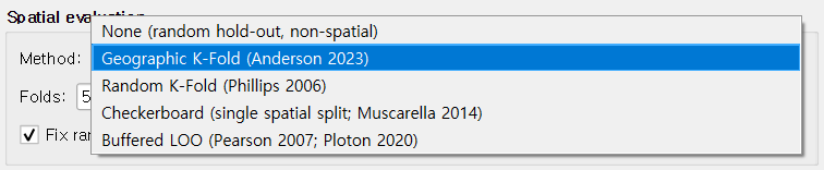
The default Geographic K-Fold (k = 5, fixed seed = 0) strikes a balance recommended by Roberts et al. 2017: geographic blocks break the spatial-autocorrelation cheating that random K-Fold permits, yet keep the held-out folds large enough for a stable AUC.

The fixed seed makes every run bit-for-bit reproducible — a property cited as essential by the SDM-best-practice review of Araújo et al. 2019.

Jackknife variable importance

When the Jackknife checkbox is on, QMaxent fits 2 × N additional single-predictor and leave-one-out models to estimate each variable's unique contribution. The cost is roughly 2 × N × training time; for the Bradypus dataset (9 variables, 116 presences) this adds about 30 seconds.

Jackknife output is rendered in two places: 1. The ④ Results → Jackknife Importance sub-tab as a paired-bar plot. 2. Table 4 of the exported XLSX workbook, with all four AUC columns plus computed Train AUC drop and Test AUC drop.

The interpretation follows the original Phillips, Anderson & Schapire 2006 reading: "with-only" bars show univariate signal; "without" bars show how dependent the full model is on each variable.

Output paths

Two file paths default to a qmaxent_output/ subdirectory of the current QGIS project:

• Model file (.pkl) — the serialised trained model, reloadable from the Data tab. See Saving and reusing models for the security note on Python pickle files.
• Results workbook (.xlsx) — multi-sheet supplementary table. See Exporting results for the sheet-by-sheet layout.

Clear either field to skip writing that file. The model object remains in memory for the rest of the session even when not saved to disk.

Advanced options

A collapsible Advanced section exposes:

• Background sample seed — separate from the CV seed, this fixes the pseudo-random draw of background points so the same study is reproducible even when the user changes the CV scheme.
• Down-weight spatially clustered points — applies the Phillips et al. 2009 sample-bias correction by giving duplicates and very-near-duplicate occurrences less weight in the likelihood. Recommended whenever the presence layer was assembled from ad-hoc records (museum specimens, citizen-science sightings, etc.).
• Add presences to background — on by default, matching Java MaxEnt convention. Required for the Maxent likelihood to be well-defined (Phillips & Dudík 2008).

Next

When everything is configured, click ▶ Run Maxent at the dock footer. Focus shifts to the ③ Training tab.