Pitta nympha

The fairy pitta Pitta nympha is a long-distance migratory passerine that breeds in dense, multi-strata broadleaved forest. The dataset shipped here reproduces a published field study — Lee et al. (2025, Global Ecology and Conservation 60:e03939) — that surveyed nest sites on Geoje Island (Geoje-si, South Korea) and trained a Maxent model with maxnet R (ENMeval 2.0). Re-running the same data in QMaxent serves two purposes:

1. Worked example for real, small-n field data (47 nest locations) with a mix of continuous topographic variables and a categorical forest-age class.
2. Cross-implementation comparison with maxent.jar — see § 3.3 of the accompanying manuscript for the formal IWLR ↔ coordinate- descent equivalence numbers (Default β=1 and Lee-matched β=4).

1. Dataset

Layer	Type	Description
pitta_nympha_occurrence	Vector point	47 nest locations on Geoje Island
TWI	Continuous raster	Topographic wetness index
TIN	Continuous raster	Terrain ruggedness
ASPECT	Continuous raster	Aspect (degrees, sin-cos pre-processed)
SLOPE	Continuous raster	Slope (°)
SMI	Continuous raster	Soil moisture index
AGE	Categorical raster	Forest age class (1–4)
DBH	Continuous raster	Mean trunk diameter at breast height
HEIGHT	Continuous raster	Mean canopy height
CANOPY_COVER	Continuous raster	Canopy closure (%)
SPECIES	Continuous raster	Dominant tree species (numeric code)

All ten rasters share a common grid (EPSG:5186 KGD2002 / Central Belt, 10 m × 10 m). This is real survey-data: the dataset is not bundled with the plugin's Example Dataset Downloader; the corresponding author of the manuscript holds the canonical copy (contact bhyu@knps.or.kr).

2. Loading data

On ① Data, pick pitta_nympha_occurrence from the Presence Points Layer drop-down (47 points), add all ten rasters from the project, mark AGE as [categorical], and click Check Raster Consistency:

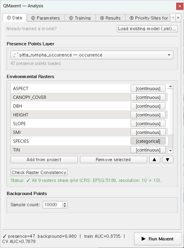
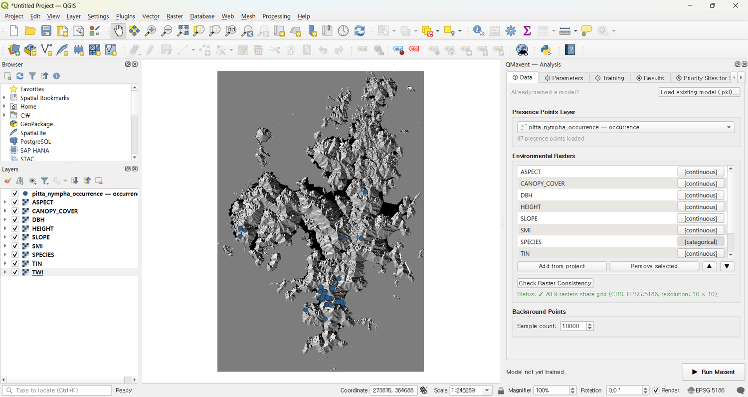
The status line reads ✓ All 10 rasters share grid (CRS: EPSG:5186, resolution: 10 × 10). The presence points cluster on Geoje Island's central forested ridges:

3. Lee-matched parameters

On ② Parameters, switch to Manual selection for Feature Types and tick Linear, Quadratic, Hinge (un-tick Product and Threshold). Set Regularization multiplier = 4.00. For Spatial evaluation, choose Random K-Fold (Phillips 2006) with Folds = 10 and seed = 42. Leave Jackknife and Permutation importance enabled (10 repeats):

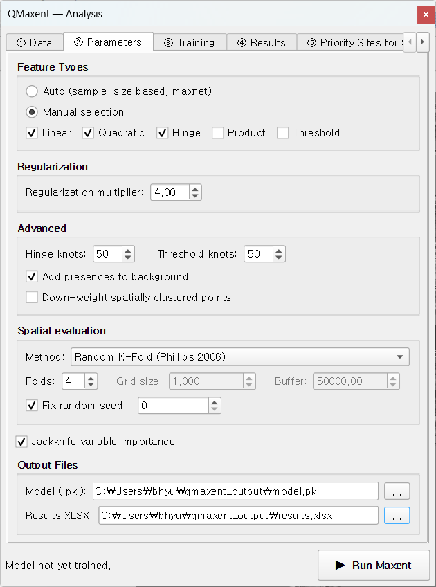
This configuration is the one ENMeval selected as optimal in Lee et al. (2025) and the one labelled "Lee-matched" in § 3.3 of the accompanying manuscript. Re-running it under maxent.jar v3.4.4 on the same data yields the maxent.jar side of the comparison (Training AUC = 0.8692 ± 0.0230, 10-fold CV AUC = 0.8128 ± 0.1022) — within the |Δ| < 0.005 micro-convergence band documented for IWLR ↔ coordinate-descent in § 2.3.

4. Training

Click ▶ Run Maxent. The Training tab finishes in ~ 20 seconds:

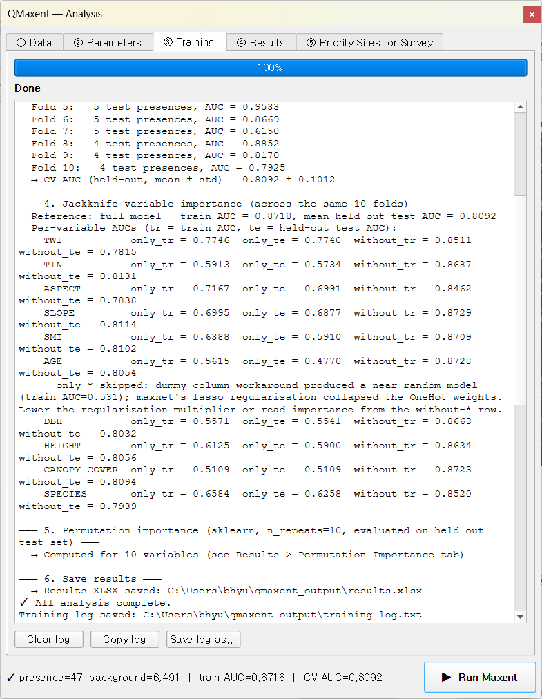
The status bar at the bottom reads presence=47 background=6,491 | train AUC=0.8718 | CV AUC=0.8092.

• Full-data model — Training AUC = 0.8718 (QMaxent side of the manuscript's Table 3 Lee-matched row; maxent.jar = 0.8692, |Δ| = 0.0026, well within the 0.005 tolerance band).
• Cross-validation — Random K-Fold n=10, seed=42. Pooled mean ± std = 0.8092 ± 0.1012. Per-fold AUCs visible in the log range from 0.6150 to 0.9533 — a wider spread than Bradypus or Ariolimax, reflecting the small sample (4–5 test presences per fold) typical of field-survey datasets.

Jackknife with a categorical variable

The log surfaces a useful diagnostic that does not appear in the Bradypus / Ariolimax runs:

only-* skipped: dummy-column workaround produced a near-random model (train AUC = 0.531); maxnet's lasso regularisation collapsed the OneHot weights. Lower the regularization multiplier or read importance from the without-* row.

AGE is the only categorical variable in the stack. In the only- this-variable jackknife pass it must be one-hot encoded, but at β = 4 the L1 lasso penalty collapses every OneHot weight back to near-zero — Maxent has nothing left to score with. QMaxent detects this collapse, skips the affected only-* row, and tells you in plain English. The without-* row remains informative and is the right place to read AGE's incremental contribution.

This is exactly the over-regularisation failure mode Merow et al. 2013 describe. The β = 1 Default run (not shown here) recovers a meaningful only-AGE AUC.

5. Variable behaviour

Response curve — ASPECT

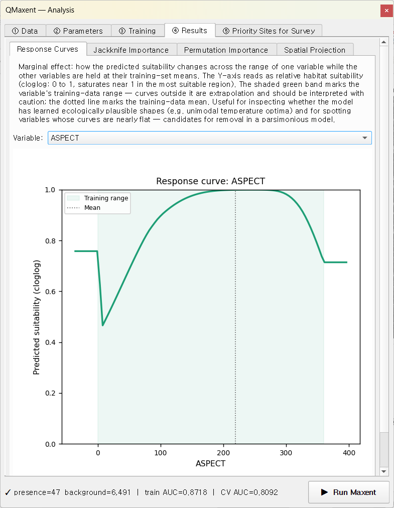
The model assigns highest suitability to north-facing aspects (roughly 270°–360°), consistent with the fairy pitta's known preference for shaded, cool, humid microclimates on ridge shoulders.

Jackknife importance

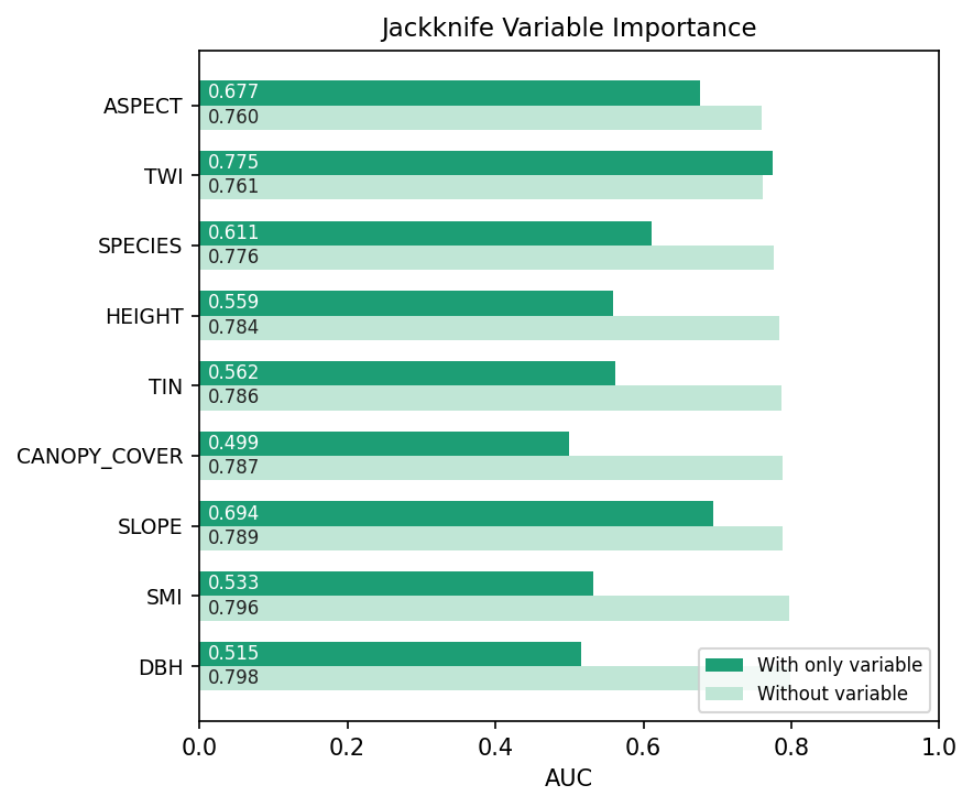
ASPECT, TWI, and SPECIES carry the strongest without-row signals — removing them costs the most. AGE's only-* bar is absent for the reason described in § 4 above; its without-* ranking (~ 0.81) places it mid-pack, which is the honest reading.

Permutation importance

The permutation pass evaluates each variable on the held-out test set independent of the lasso shrinkage that disabled AGE's only-* row, so all ten variables get a comparable percentage:

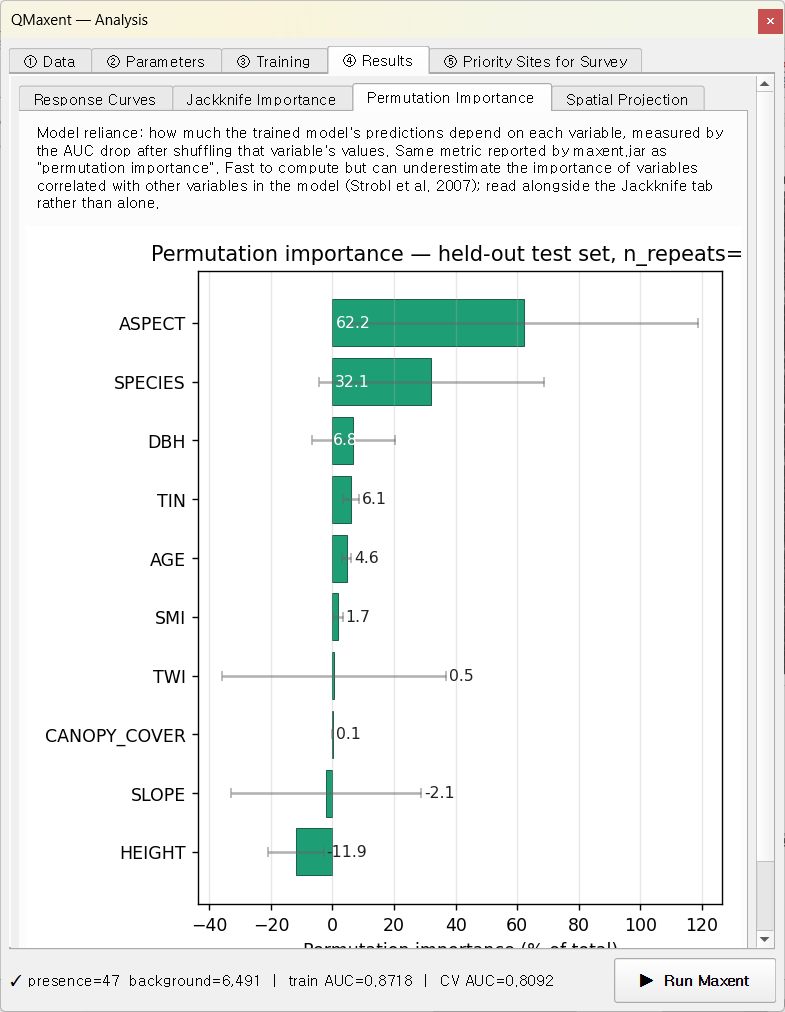
The agreement between Jackknife without-* and Permutation rankings (Spearman ρ at this β = 4 configuration is small, see manuscript § 3.3) reflects the over-regularisation effect rather than an implementation bug.

6. Priority sites for survey

After projection, the ⑤ Priority Sites for Survey → Discovery mode produces field-trip candidates on Geoje. Because the study area is much smaller than Bradypus or Ariolimax, the suitability threshold (~ 0.88) and spacing rules (1 km from existing presences, 500 m between candidates) yield a tractable list of about twenty new search locations:

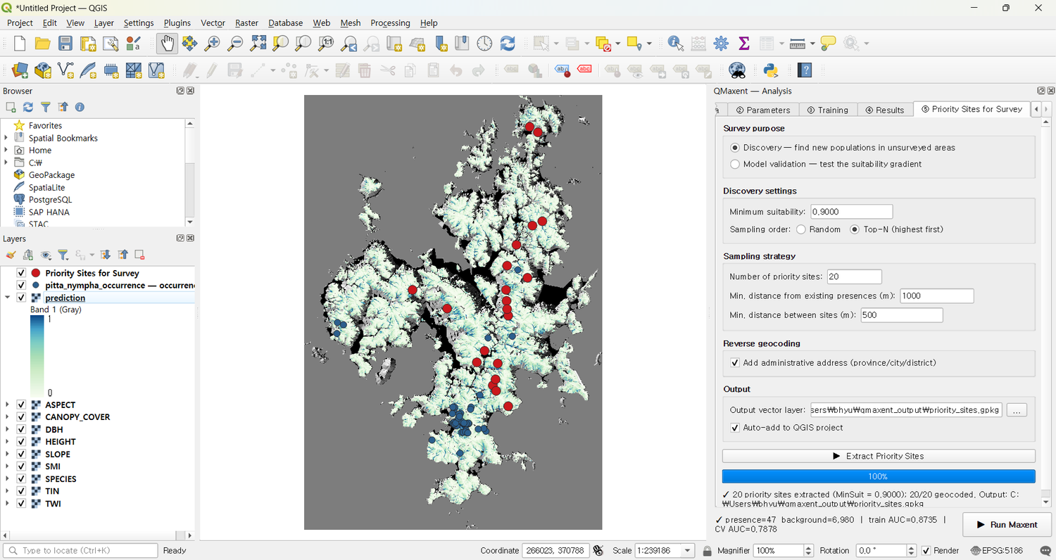
Nominatim reverse geocoding populates the attribute table with administrative names down to eup/myeon/dong level where available — a one-step path from model to field-trip planning.

7. What this example demonstrates

1. Real-data workflow with small-n field surveys (47 presences, 10 covariates, real-world spatial scale).
2. Categorical variable handling plus the OneHot-collapse diagnostic when over-regularised.
3. The Lee-matched (β = 4) configuration that the accompanying manuscript uses for its maxent.jar numerical-compatibility benchmark (§ 3.3 / Table 3).
4. A different, narrower kind of priority-sites use-case — targeted re-survey of known sub-populations rather than continental discovery.

For the formal maxent.jar ↔ QMaxent comparison numbers (Training AUC |Δ| < 0.005, permutation-importance Spearman ρ at both β=1 and β=4) see the accompanying manuscript's § 3.3 and the JSON record under tests/fixtures/pitta_golden_values.json.