Ariolimax
The Pacific banana slug Ariolimax columbianus is the second worked example. Its purpose is different from Bradypus's feature tour — this dataset is deliberately messy: the supplied environmental rasters do not share a common CRS, extent, or resolution. The example walks through QMaxent's Check Raster Consistency preflight and Harmonize to Folder… workflow, showing the silent-failure mode you would otherwise hit and the one-click fix that makes the data Maxent-ready.
1. Dataset
The Ariolimax dataset is the default that ships with elapid. It comes in two variants chosen via the Download Example Dataset dialog:
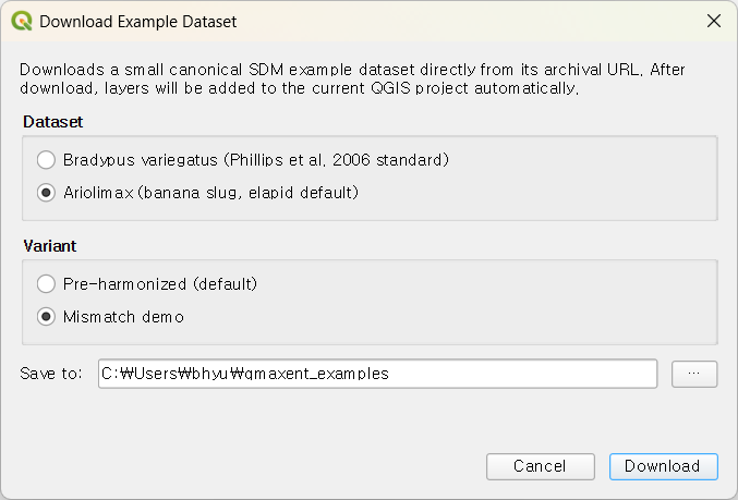
- Pre-harmonized (default) — the same six rasters already reprojected and resampled onto a common grid. Use this if you want to jump straight to model fitting.
- Mismatch demo — the original tiles with their original CRS, extent, and resolution intact. Use this if you want to exercise the Check + Harmonize tooling.
This walkthrough uses the Mismatch demo variant. After clicking Download, the layers appear on the QGIS canvas spanning California's coastal range:
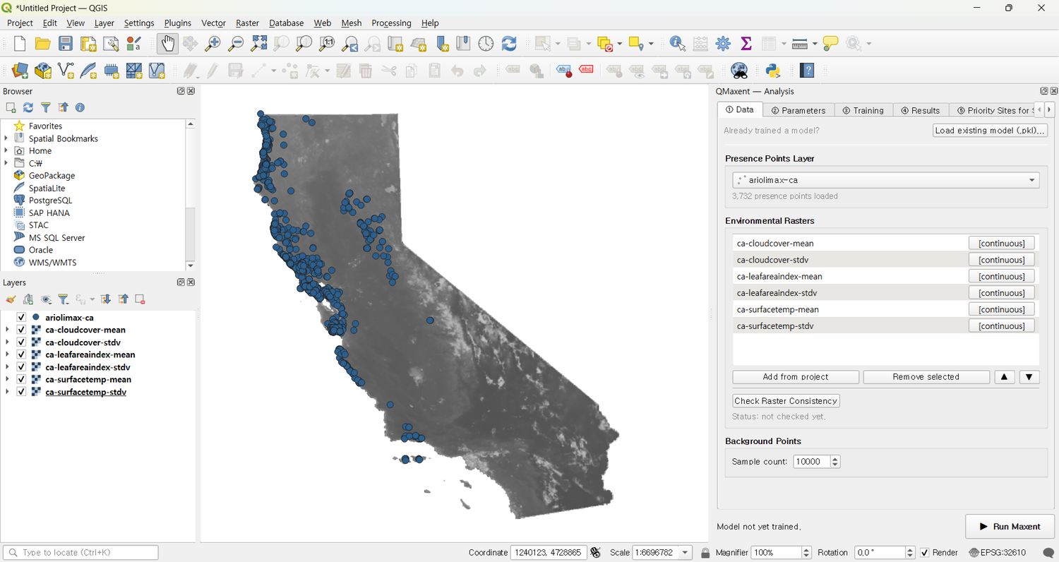
Visually the data already looks unified. The raster tiles, however, were authored by different remote-sensing pipelines and inherit different projections and resolutions — exactly the situation that breaks Maxent silently.
2. The mismatch problem
Open Plugins → QMaxent → QMaxent Analysis. On ① Data, choose
the ariolimax-ca presence layer (3,732 points), then Add from
project to register every loaded raster (six in total —
ca-cloudcover-mean, ca-cloudcover-stdv, ca-leafareaindex-mean,
ca-leafareaindex-stdv, ca-surfacetemp-mean, ca-surfacetemp-stdv).
Click Check Raster Consistency:
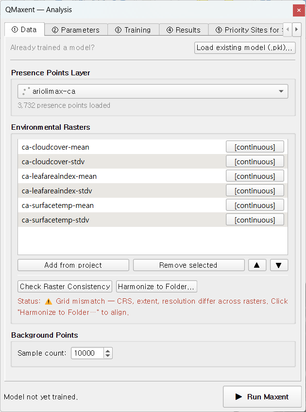
The status line turns amber and reports:
⚠ Grid mismatch — CRS, extent, resolution differ across rasters. Click "Harmonize to Folder…" to align.
Crucially, the Run Maxent button is not blocked — Maxent itself would still produce numbers. Those numbers, however, would be silently wrong: covariates would be sampled from the cells nominally underneath each presence point but actually belonging to misaligned rasters. This is the single most common silent-failure mode in operational SDM and the entire reason this preflight exists.
3. Running Harmonize to Folder…
A new button appears next to Check Raster Consistency as soon as a
mismatch is detected: Harmonize to Folder…. Click it and choose
an output directory. QMaxent picks the highest-resolution raster
as the reference grid, reprojects every other raster to that grid via
gdalwarp under the hood
(nearest-neighbour for categoricals, bilinear for continuous), and
writes new GeoTIFFs into the chosen folder. The new files are
auto-loaded into the project and the old ones are removed from the
QMaxent raster list.
The Data tab refreshes to show the harmonized stack:
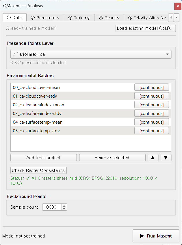
The status line is now green:
✓ All 6 rasters share grid (CRS: EPSG:3857, resolution: 1258.3 × 1258.3).
Harmonized rasters get a numeric prefix (00_, 01_, …) that locks
their order. This survives a .qgz save+reload cycle — the model
variable order is part of the model's identity, and the prefix makes
that order visible at the file-system level too.
4. Running the model
With the stack harmonized, the rest of the workflow is identical to Bradypus. Accept the defaults on ② Parameters, click ▶ Run Maxent, and let the training complete:
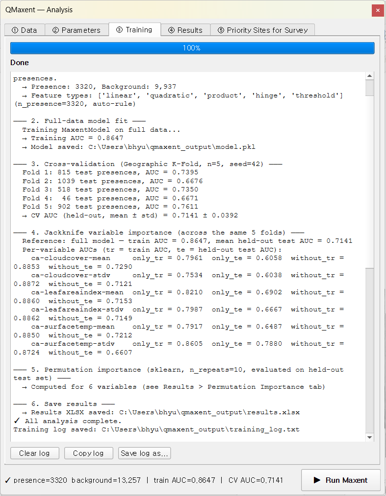
The status bar at the bottom summarises:
presence=3320 background=13,257 | train AUC=0.8647 | CV AUC=0.7141.
Reading the log:
- Full-data model —
Training AUC = 0.8647. - Cross-validation — Geographic K-Fold n=5, seed=42:
| Fold | Test presences | AUC |
|---|---|---|
| 1 | 815 | 0.7395 |
| 2 | 1,039 | 0.6676 |
| 3 | 518 | 0.7350 |
| 4 | 46 | 0.6671 |
| 5 | 902 | 0.7611 |
Pooled mean ± std = 0.7141 ± 0.0392.
The much tighter ± 0.04 standard deviation (compared to Bradypus's ± 0.075) reflects Ariolimax's larger and more uniformly distributed presence sample — when each spatial fold contains hundreds rather than a handful of presences, the per-fold AUC stabilises.
5. Variable behaviour
Response curve
ca-surfacetemp-stdv (variability of land-surface temperature)
carries the strongest stand-alone signal — biologically sensible for
an organism whose activity windows depend on cool, moist
microclimates:
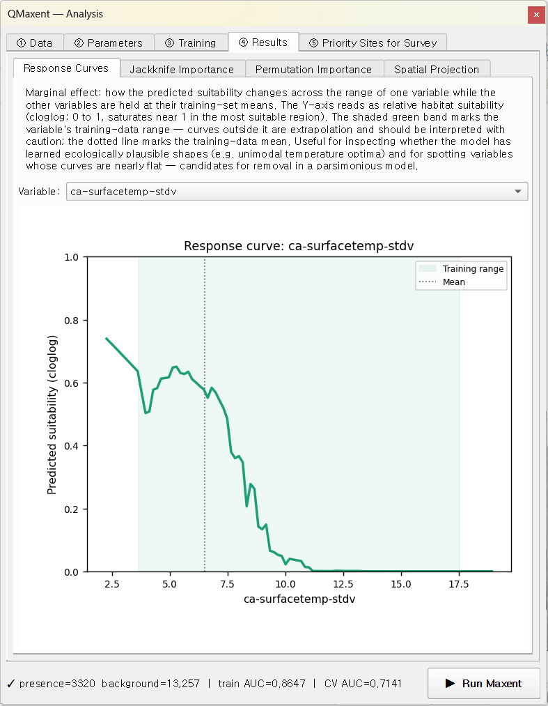
The curve shows suitability rising as temperature variability falls below ~ 2 K and dropping to near zero above ~ 8 K — the classic preference of a moisture-dependent species for thermally stable maritime climates.
Jackknife importance
The Jackknife panel ranks every variable by both stand-alone power and removal cost:
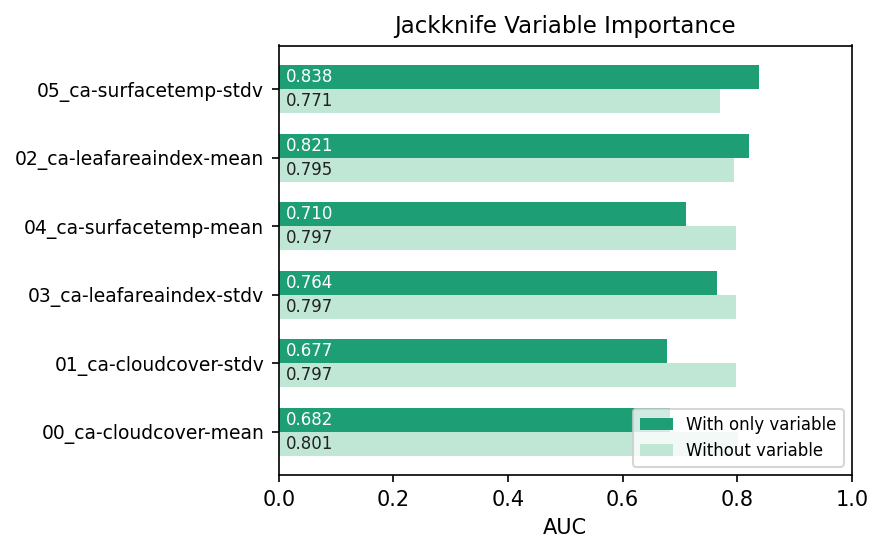
ca-surfacetemp-stdv and ca-leafareaindex-mean lead, with the
cloud-cover variables weakest. The "without" bars cluster tightly
above 0.85 — same correlation-pattern argument as Bradypus.
Permutation importance
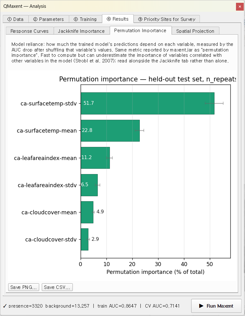
The permutation view distributes the total importance across all variables and is directly comparable to maxent.jar's per-variable percentage table:
6. Comparing models with and without harmonization
We strongly recommend running the model once on the unharmonized stack as a teaching exercise. With Maxent's permissive raster handling you will get a finished model and a finished AUC, but the AUC will typically be 0.05–0.10 higher than the harmonized run — not because the model is better, but because covariate misalignment introduces spurious patterns that the model fits to. The cross-validation gap (training vs. CV AUC) widens correspondingly.
Always run Check Raster Consistency before drawing conclusions.
7. Priority sites for survey
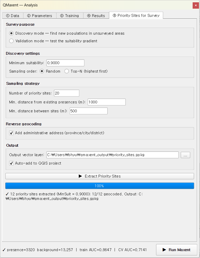
After projection, switch to ⑤ Priority Sites for Survey, choose Discovery mode, and extract candidates. The defaults work well for Ariolimax's smaller study area:
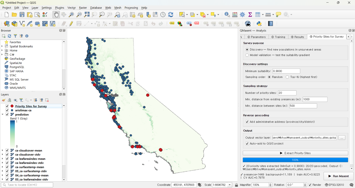
The sites land on the coastal mountain ranges that the suitability map highlighted, and survey teams can take the resulting GeoPackage straight to the field:
What this example demonstrates
- The two example variants (Pre-harmonized vs Mismatch demo) for didactic use of the same dataset.
- The silent-failure mode of Maxent when rasters disagree.
- QMaxent's preflight + harmonize tooling that turns a project-killing mistake into a one-click fix.
- Sample-size effects on spatial CV variability — 3,732 presences produce a tighter ± std than Bradypus's 116.
Carry the same habit into your own work: every time you assemble a new raster stack, run Check Raster Consistency before training. If it fails, harmonize first, train second.