Quick start
This 5-minute walkthrough takes you from a freshly installed plugin to a finished habitat-suitability map for Bradypus variegatus, the brown-throated three-toed sloth — the same species the original Maxent paper used Phillips, Anderson & Schapire 2006. Every screenshot below shows real numbers from a run you can reproduce.
Prerequisites
Make sure you have completed Installation and Dependencies — the QMaxent environment ready banner must be green before continuing.
Step 1 · Download the example dataset
Open Plugins → QMaxent → Download Example Dataset, choose Bradypus variegatus, and confirm.
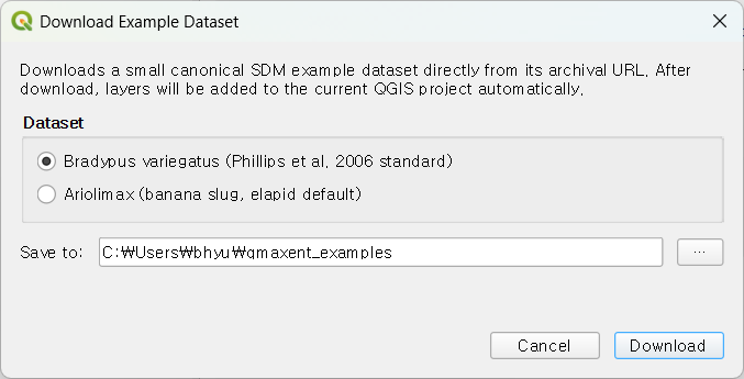
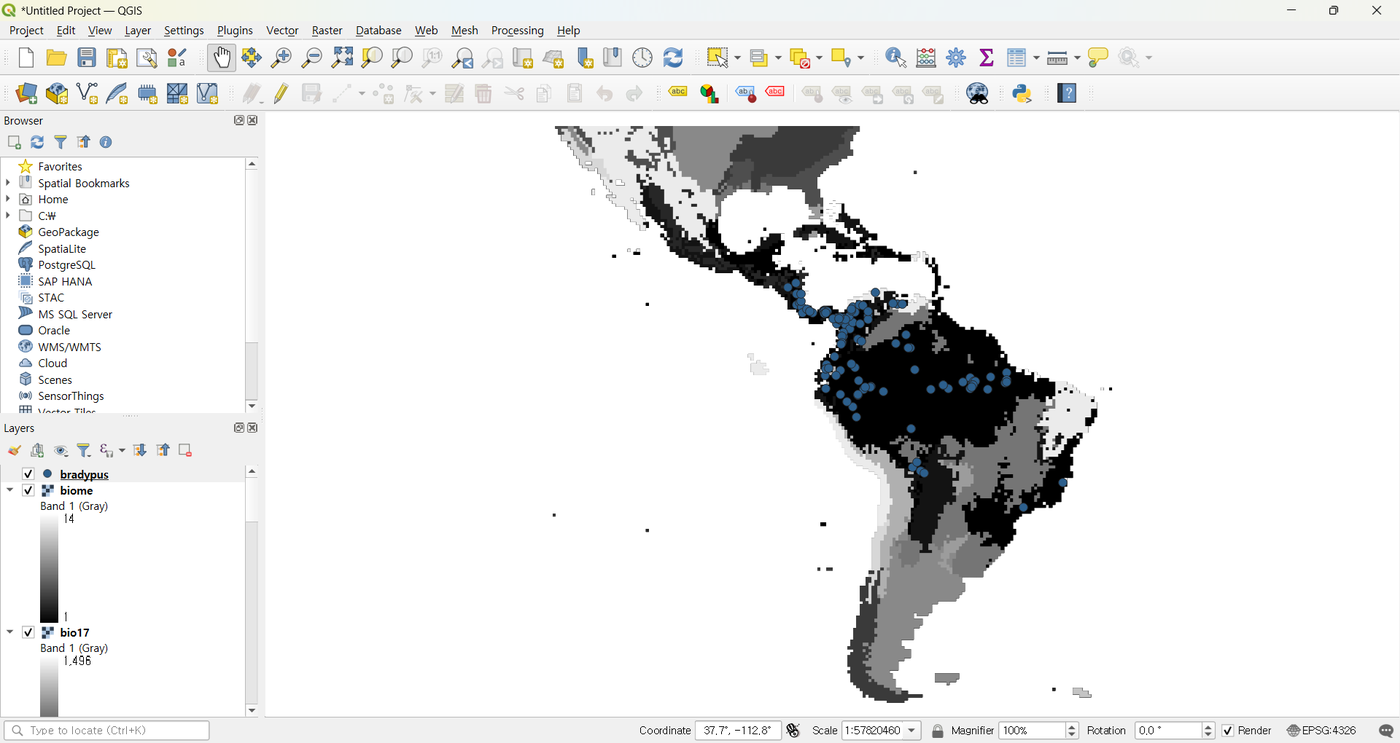
QMaxent fetches the bundled dataset (presence shapefile + 9 environmental rasters at 0.5° resolution covering the Americas) and adds every layer to the active QGIS project automatically.
Step 2 · Open the Analysis dock
Choose Plugins → QMaxent → QMaxent Analysis. The dock opens on the right of the QGIS main window with five numbered tabs you progress through left-to-right.
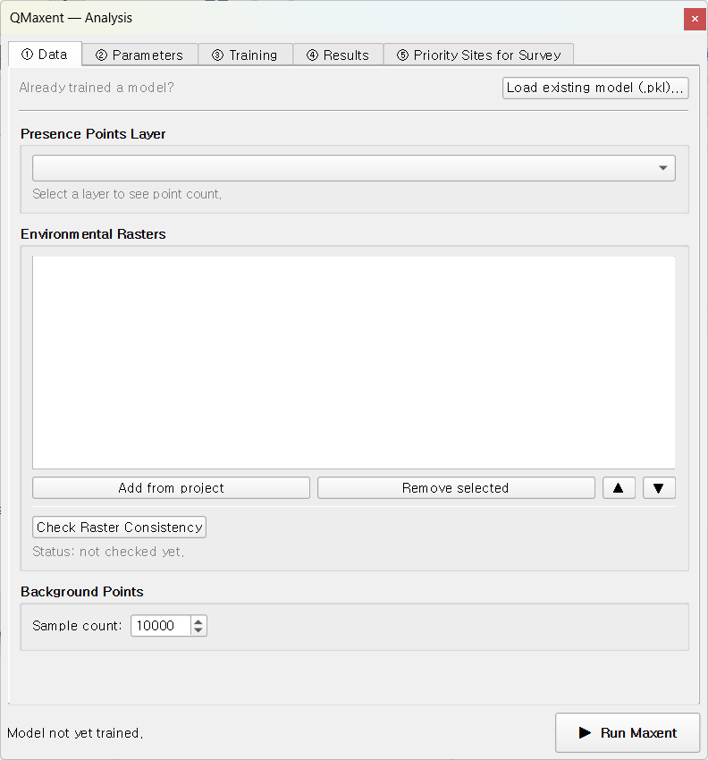
Step 3 · Configure the Data tab
On ① Data, pick bradypus from the Presence Points Layer drop-down
(QMaxent reports 116 presence points loaded), click Add from project
to register every loaded raster at once, then click Check Raster
Consistency to verify the stack.
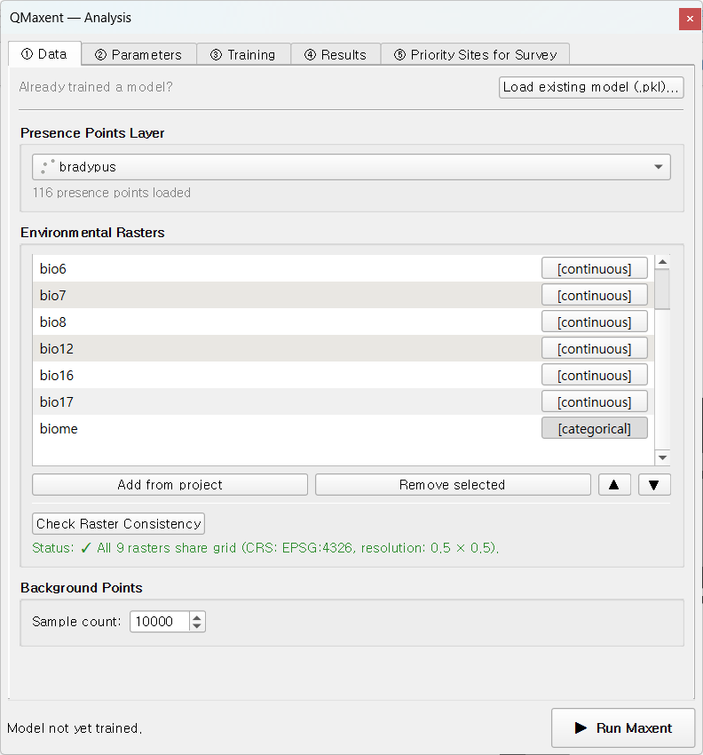
The status line should turn green:
✓ All 9 rasters share grid (CRS: EPSG:4326, resolution: 0.5 × 0.5).
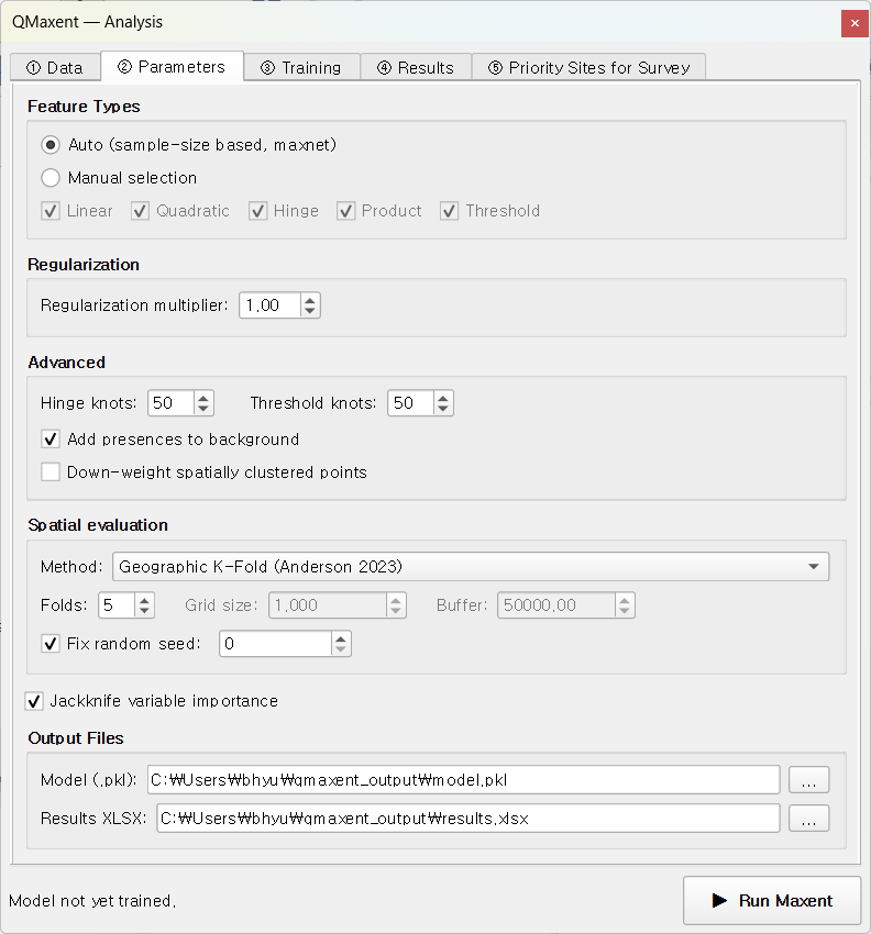
Step 4 · Accept the Parameters defaults
Switch to ② Parameters. For this quick tour, every default is deliberately the recommended setting from the SDM literature (Phillips & Dudík 2008, Radosavljevic & Anderson 2014):
- Feature classes: Auto (the maxnet rule that follows Phillips & Dudík 2008 picks LQPHT for any sample size ≥ 80)
- Regularization multiplier: 1.0
- Spatial CV: Geographic K-Fold, 5 folds, fixed seed 0
- Jackknife variable importance: enabled
- Output files:
qmaxent_output/model.pklandqmaxent_output/results.xlsx
The fixed random seed is what lets a reviewer reproduce your numbers bit-for-bit — central to the principle of computational reproducibility emphasised in the SDM-best-practice review of Araújo et al. 2019.
Step 5 · Run Maxent
Click ▶ Run Maxent at the bottom of the dock. Focus shifts to the ③ Training tab; about 30 seconds later you should see:
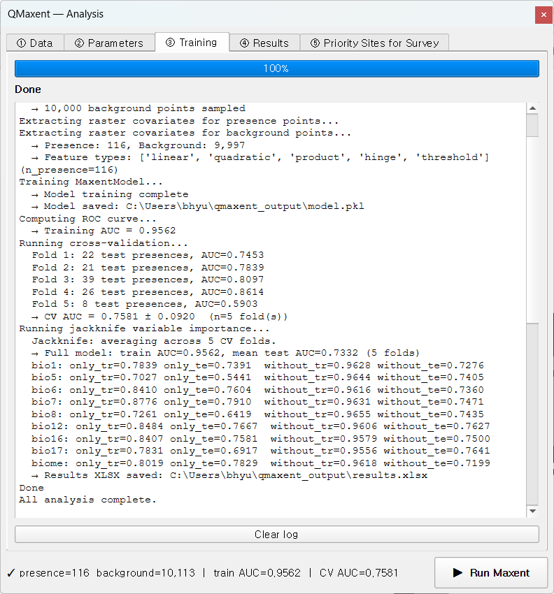
The log reports Training AUC = 0.9569 and a 5-fold mean
CV AUC = 0.7436 ± 0.0750. The honest gap between training and CV AUC is
itself a good sign — it tells you the model has not been silently
over-fitted to the training presences (a risk that
Roberts et al. 2017 document at length).
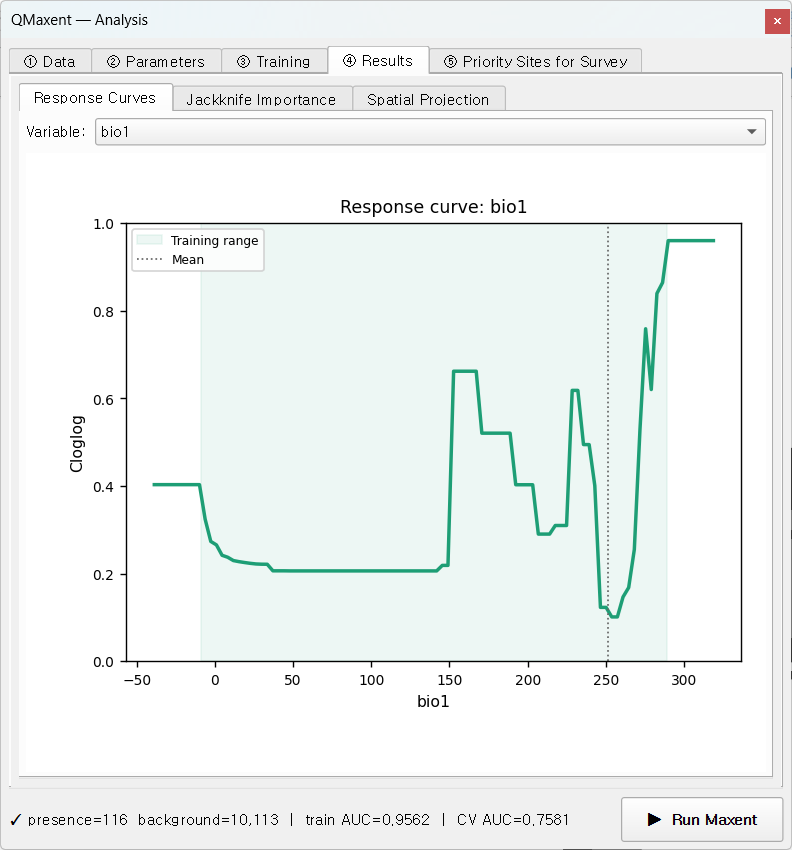
Step 6 · Inspect Response Curves and Jackknife
On ④ Results → Response Curves, pick bio1 from the variable selector
to see how the model's cloglog suitability responds to mean annual
temperature across its training range.
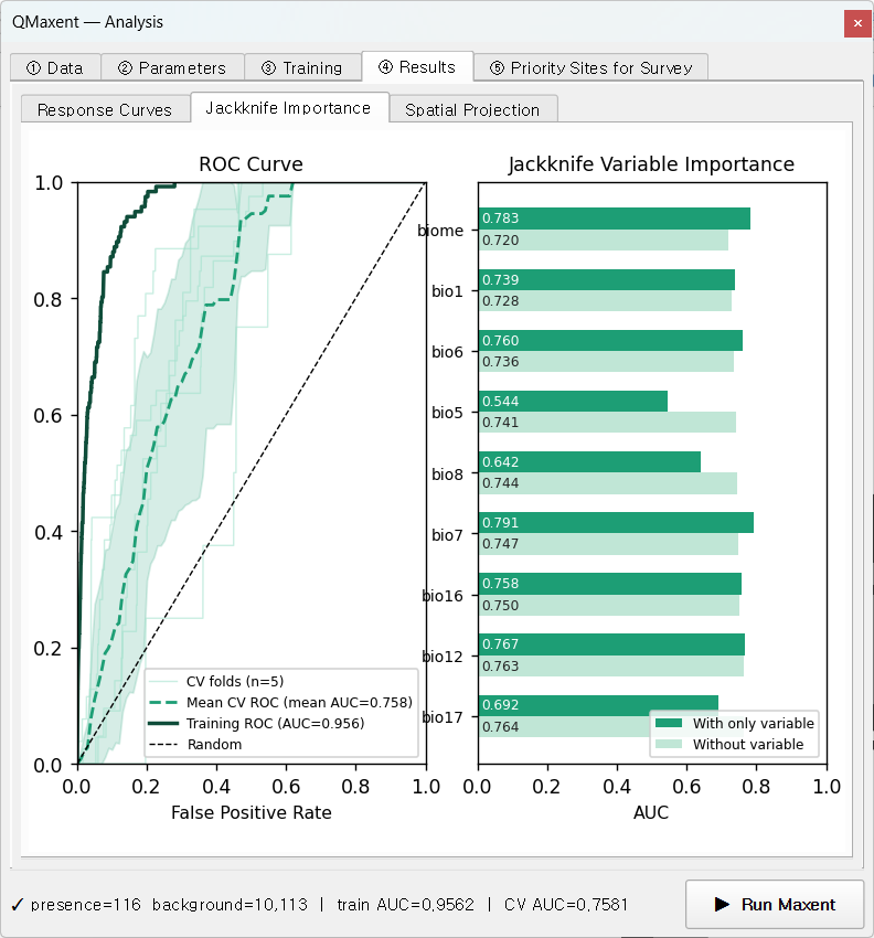
The Jackknife Importance sub-tab combines the ROC curve with per-variable contribution bars — the classic single-figure summary used in Maxent papers since Phillips, Anderson & Schapire 2006.
Step 7 · Project across the landscape
Switch to Spatial Projection. Leave cloglog as the output transform (Phillips et al. 2017 recommend cloglog as the default probability-of-presence interpretation) and Auto-load result as QGIS layer ticked, then click ▶ Run Spatial Projection.
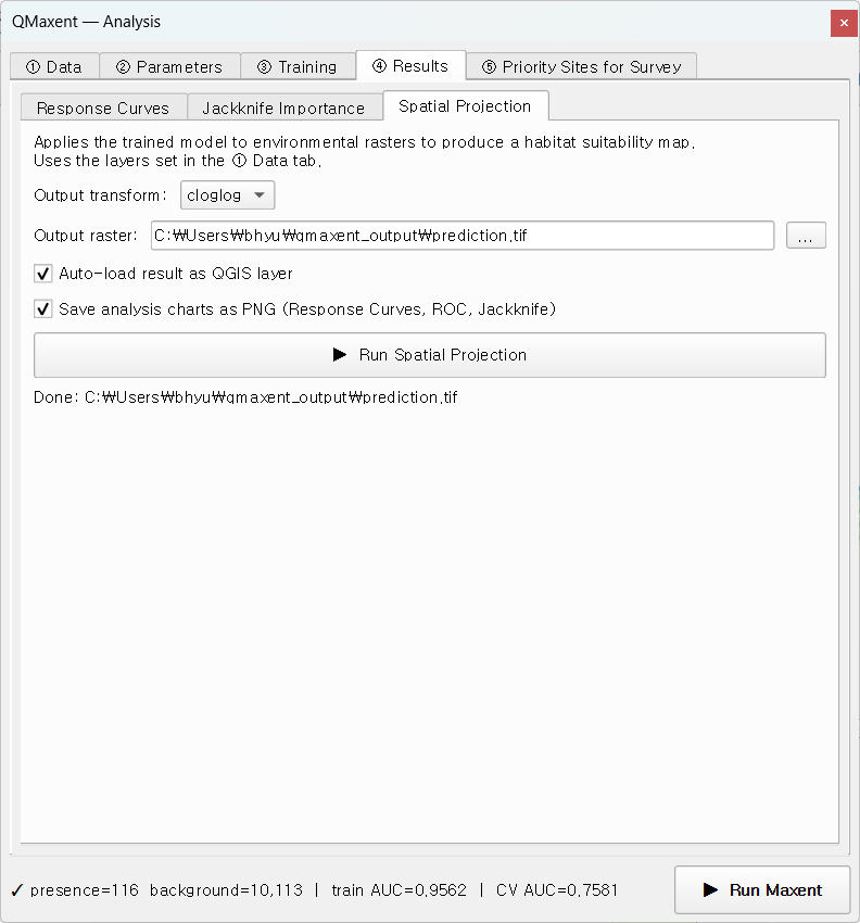
The styled GeoTIFF appears on the canvas:
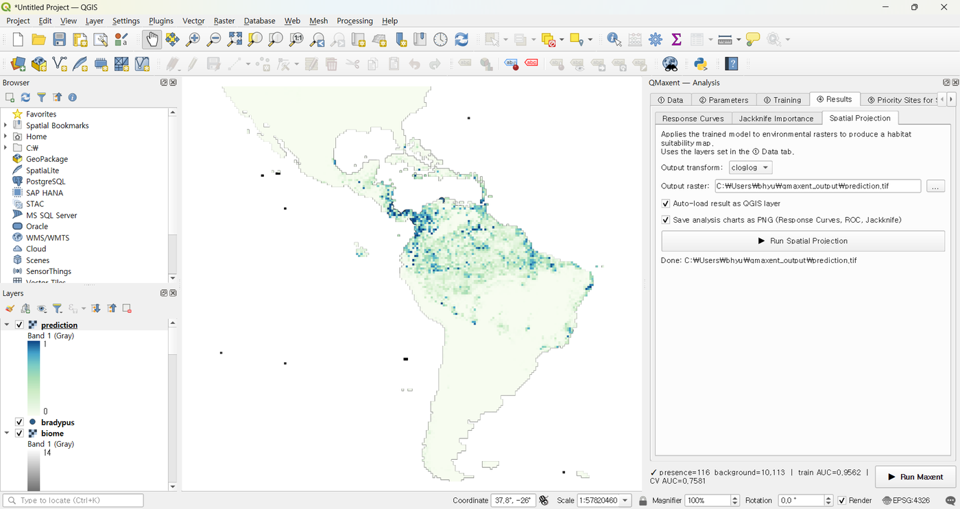
That is your finished QMaxent baseline.
What just happened
In seven clicks you ran a complete species-distribution-model pipeline: sampled background points, fit a regularized Maxent model with auto-selected features, evaluated it with spatial K-Fold CV, computed Jackknife variable importance, and projected the model across the entire dataset extent.
Next steps
- Read the User guide chapters in order to understand what each tab control does and when to override its default.
- Try the Bradypus worked example for the same workflow with deeper interpretation of every plot.
- Move to messy data with the Ariolimax example, which intentionally breaks raster alignment so you can practise the Check Raster Consistency + Harmonize to Folder… preflight.
- Reproduce a published study with the Pitta nympha example, which mirrors Lee et al. 2025 one parameter at a time.